
RatingRealities: Unveiling Bias in Movie Ratings
The story about a method for attracting more users to watch movies on a movie platform.
Overview
If you are planning on going out to see a movie, how well can you trust online reviews and ratings? Especially if the same company showing the rating also makes money by selling movie tickets. Do they have a bias towards rating movies higher than they should be rated?
Goal:
Goal is to analyse movie data based on the 538 article (Be Suspicious Of Online Movie Ratings, Especially Fandango’s) and see if concnclusions are similar. I am going to use pandas and visualization skills to determine if Fandango’s ratings in 2015 had a bias towards rating movies better to sell more tickets.
Part One: Understanding the Background and Data
The Data
This is the data behind the story Be Suspicious Of Online Movie Ratings, Especially Fandango’s openly available on 538’s github: https://github.com/fivethirtyeight/data. There are two csv files, one with Fandango Stars and Displayed Ratings, and the other with aggregate data for movie ratings from other sites, like Metacritic,IMDB, and Rotten Tomatoes.
all_sites_scores.csv
all_sites_scores.csv contains every film that has a Rotten Tomatoes rating, a RT User rating, a Metacritic score, a Metacritic User score, and IMDb score, and at least 30 fan reviews on Fandango. The data from Fandango was pulled on Aug. 24, 2015.
| Column | Definition |
|---|---|
| FILM | The film in question |
| RottenTomatoes | The Rotten Tomatoes Tomatometer score for the film |
| RottenTomatoes_User | The Rotten Tomatoes user score for the film |
| Metacritic | The Metacritic critic score for the film |
| Metacritic_User | The Metacritic user score for the film |
| IMDB | The IMDb user score for the film |
| Metacritic_user_vote_count | The number of user votes the film had on Metacritic |
| IMDB_user_vote_count | The number of user votes the film had on IMDb |
fandango_scape.csv
fandango_scrape.csv contains every film 538 pulled from Fandango.
| Column | Definiton |
|---|---|
| FILM | The movie |
| STARS | Number of stars presented on Fandango.com |
| RATING | The Fandango ratingValue for the film, as pulled from the HTML of each page. This is the actual average score the movie obtained. |
| VOTES | number of people who had reviewed the film at the time we pulled it. |
Part Two: Exploring Fandango Displayed Scores versus True User Ratings
Checkpoint 1. Let’s first explore the Fandango ratings to see if our analysis agrees with the article’s conclusion.
import pandas as pd
import matplotlib.pyplot as plt
import seaborn as sns
import numpy as np
fandango = pd.read_csv("fandango_scrape.csv")
Fandango’s table structure
fandango.head()
| FILM | STARS | RATING | VOTES | |
|---|---|---|---|---|
| 0 | Fifty Shades of Grey (2015) | 4.0 | 3.9 | 34846 |
| 1 | Jurassic World (2015) | 4.5 | 4.5 | 34390 |
| 2 | American Sniper (2015) | 5.0 | 4.8 | 34085 |
| 3 | Furious 7 (2015) | 5.0 | 4.8 | 33538 |
| 4 | Inside Out (2015) | 4.5 | 4.5 | 15749 |
Fandango’s table information
fandango.info()
<class 'pandas.core.frame.DataFrame'>
RangeIndex: 504 entries, 0 to 503
Data columns (total 4 columns):
 #   Column  Non-Null Count  Dtype
---  ------  --------------  -----
 0   FILM    504 non-null    object
 1   STARS   504 non-null    float64
 2   RATING  504 non-null    float64
 3   VOTES   504 non-null    int64
dtypes: float64(2), int64(1), object(1)
memory usage: 15.9+ KB
Fandango descriptive statistics
fandango.describe().transpose()
| count | mean | std | min | 25% | 50% | 75% | max | |
|---|---|---|---|---|---|---|---|---|
| STARS | 504.0 | 3.558532 | 1.563133 | 0.0 | 3.5 | 4.0 | 4.50 | 5.0 |
| RATING | 504.0 | 3.375794 | 1.491223 | 0.0 | 3.1 | 3.8 | 4.30 | 5.0 |
| VOTES | 504.0 | 1147.863095 | 3830.583136 | 0.0 | 3.0 | 18.5 | 189.75 | 34846.0 |
Checkpoint 2. Exploring the relationship between popularity of a film and its rating.
plt.figure(figsize=(12,4))
sns.scatterplot(data=fandango, x="RATING", y="VOTES")
plt.title("Relationship between popularity and films' rating")
Text(0.5, 1.0, "Relationship between popularity and films' rating")
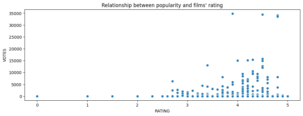
Correlation matrix
fandango[["STARS","RATING","VOTES"]].corr()
| STARS | RATING | VOTES | |
|---|---|---|---|
| STARS | 1.000000 | 0.994696 | 0.164218 |
| RATING | 0.994696 | 1.000000 | 0.163764 |
| VOTES | 0.164218 | 0.163764 | 1.000000 |
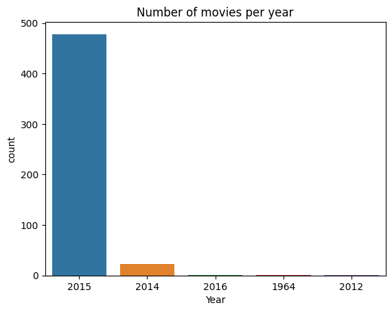
Checkpoint 3. Frequency analysis.
# Separating the column that contains the name and film year into a column with the year of the film
fandango['Year'] = fandango['FILM'].apply(lambda title:title.split('(')[-1].replace(')',''))
Number of movies per year
# Checking the frequency of the "Year" column
fandango["Year"].value_counts()
2015    478
2014     23
2016      1
1964      1
2012      1
Name: Year, dtype: int64
# Ploting the "Year" column
sns.countplot(data=fandango,x="Year")
plt.title("Number of movies per year")
Text(0.5, 1.0, 'Number of movies per year')
10 movies with highest number of votes
# 10 movies with highest number of votes
fandango.sort_values(by=["VOTES"], ascending=False)[:10]
| FILM | STARS | RATING | VOTES | Year | |
|---|---|---|---|---|---|
| 0 | Fifty Shades of Grey (2015) | 4.0 | 3.9 | 34846 | 2015 |
| 1 | Jurassic World (2015) | 4.5 | 4.5 | 34390 | 2015 |
| 2 | American Sniper (2015) | 5.0 | 4.8 | 34085 | 2015 |
| 3 | Furious 7 (2015) | 5.0 | 4.8 | 33538 | 2015 |
| 4 | Inside Out (2015) | 4.5 | 4.5 | 15749 | 2015 |
| 5 | The Hobbit: The Battle of the Five Armies (2014) | 4.5 | 4.3 | 15337 | 2014 |
| 6 | Kingsman: The Secret Service (2015) | 4.5 | 4.2 | 15205 | 2015 |
| 7 | Minions (2015) | 4.0 | 4.0 | 14998 | 2015 |
| 8 | Avengers: Age of Ultron (2015) | 5.0 | 4.5 | 14846 | 2015 |
| 9 | Into the Woods (2014) | 3.5 | 3.4 | 13055 | 2014 |
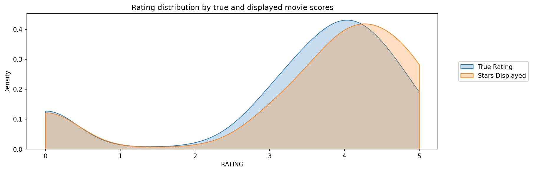
Number of movies with zero votes
# Number of movies with zero votes
fandango[fandango["VOTES"] == 0].count()["VOTES"]
69
Number of movies that have votes
# Updating DataFrame of only reviewed films
fandango = fandango[fandango["VOTES"] != 0]
len(fandango)
435
# The distributions of ratings that are dispayed (STARS) versus what the true rating was from votes (RATING)
plt.figure(figsize=(12,4), dpi=150)
sns.kdeplot(data=fandango, x="RATING", clip=(0,5), label="True Rating", fill=True)
sns.kdeplot(data=fandango, x="STARS", clip=(0,5), label="Stars Displayed", fill=True)
plt.legend(loc=(1.05,0.5))
plt.title("Rating distribution by true and displayed movie scores")
Text(0.5, 1.0, 'Rating distribution by true and displayed movie scores')
The discepancy between STARS and RATING - STARS_DIFF
# Quantifing the discepancy between STARS and RATING
fandango["STARS_DIFF"] = fandango["STARS"] - fandango["RATING"]
fandango.head()
| FILM | STARS | RATING | VOTES | Year | STARS_DIFF | |
|---|---|---|---|---|---|---|
| 0 | Fifty Shades of Grey (2015) | 4.0 | 3.9 | 34846 | 2015 | 0.1 |
| 1 | Jurassic World (2015) | 4.5 | 4.5 | 34390 | 2015 | 0.0 |
| 2 | American Sniper (2015) | 5.0 | 4.8 | 34085 | 2015 | 0.2 |
| 3 | Furious 7 (2015) | 5.0 | 4.8 | 33538 | 2015 | 0.2 |
| 4 | Inside Out (2015) | 4.5 | 4.5 | 15749 | 2015 | 0.0 |
# Displaying the number of times a certain difference occurs
plt.figure(figsize=(12,4), dpi=150)
sns.histplot(data=fandango, x="STARS_DIFF", bins=7)
plt.title("Number of times a certain difference occurs")
Text(0.5, 1.0, 'Number of times a certain difference occurs')
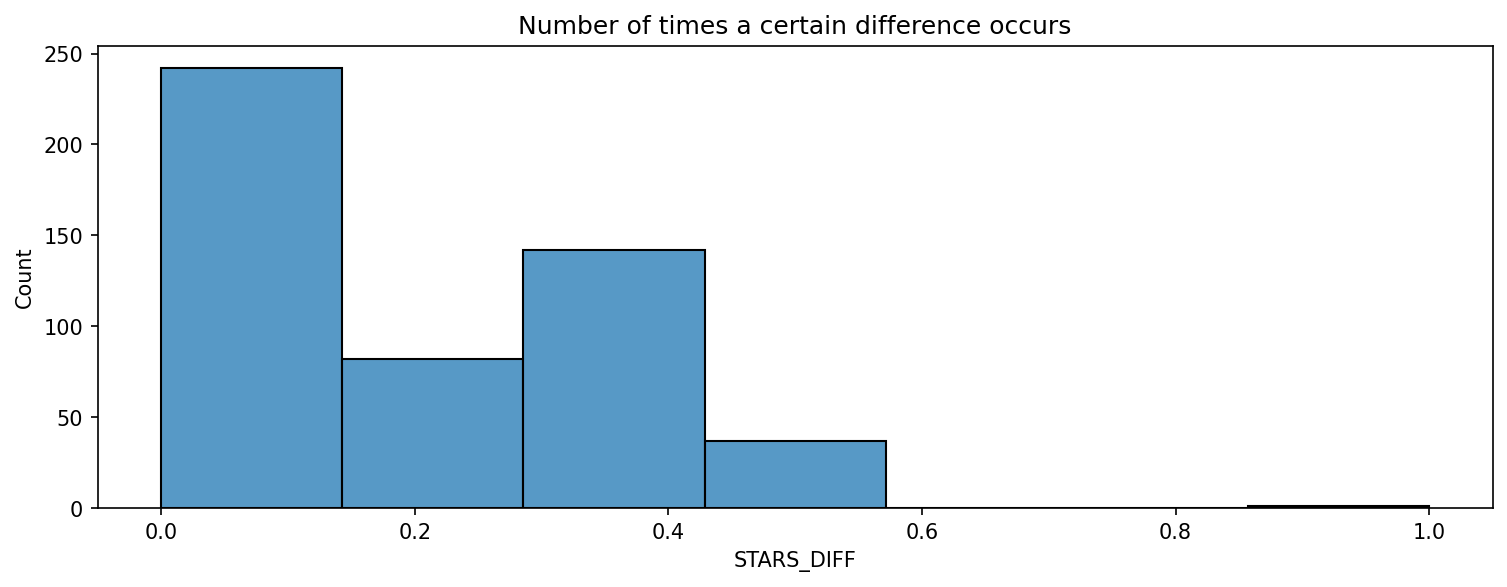
Movie that is close to 1 star differential
# Movie that is close to 1 star differential
fandango[fandango["STARS_DIFF"] == 1]
| FILM | STARS | RATING | VOTES | Year | STARS_DIFF | |
|---|---|---|---|---|---|---|
| 381 | Turbo Kid (2015) | 5.0 | 4.0 | 2 | 2015 | 1.0 |
Part Three: Comparison of Fandango Ratings to Other Sites
Let’s now compare the scores from Fandango to other movies sites and see how they compare.
all_sites = pd.read_csv("all_sites_scores.csv")
All sites table structure
all_sites.head()
| FILM | RottenTomatoes | RottenTomatoes_User | Metacritic | Metacritic_User | IMDB | Metacritic_user_vote_count | IMDB_user_vote_count | |
|---|---|---|---|---|---|---|---|---|
| 0 | Avengers: Age of Ultron (2015) | 74 | 86 | 66 | 7.1 | 7.8 | 1330 | 271107 |
| 1 | Cinderella (2015) | 85 | 80 | 67 | 7.5 | 7.1 | 249 | 65709 |
| 2 | Ant-Man (2015) | 80 | 90 | 64 | 8.1 | 7.8 | 627 | 103660 |
| 3 | Do You Believe? (2015) | 18 | 84 | 22 | 4.7 | 5.4 | 31 | 3136 |
| 4 | Hot Tub Time Machine 2 (2015) | 14 | 28 | 29 | 3.4 | 5.1 | 88 | 19560 |
All sites table info
all_sites.info()
<class 'pandas.core.frame.DataFrame'>
RangeIndex: 146 entries, 0 to 145
Data columns (total 8 columns):
 #   Column                      Non-Null Count  Dtype
---  ------                      --------------  -----
 0   FILM                        146 non-null    object
 1   RottenTomatoes              146 non-null    int64
 2   RottenTomatoes_User         146 non-null    int64
 3   Metacritic                  146 non-null    int64
 4   Metacritic_User             146 non-null    float64
 5   IMDB                        146 non-null    float64
 6   Metacritic_user_vote_count  146 non-null    int64
 7   IMDB_user_vote_count        146 non-null    int64
dtypes: float64(2), int64(5), object(1)
memory usage: 9.2+ KB
All sites descriptive statistics
all_sites.describe().transpose()
| count | mean | std | min | 25% | 50% | 75% | max | |
|---|---|---|---|---|---|---|---|---|
| RottenTomatoes | 146.0 | 60.849315 | 30.168799 | 5.0 | 31.25 | 63.50 | 89.00 | 100.0 |
| RottenTomatoes_User | 146.0 | 63.876712 | 20.024430 | 20.0 | 50.00 | 66.50 | 81.00 | 94.0 |
| Metacritic | 146.0 | 58.808219 | 19.517389 | 13.0 | 43.50 | 59.00 | 75.00 | 94.0 |
| Metacritic_User | 146.0 | 6.519178 | 1.510712 | 2.4 | 5.70 | 6.85 | 7.50 | 9.6 |
| IMDB | 146.0 | 6.736986 | 0.958736 | 4.0 | 6.30 | 6.90 | 7.40 | 8.6 |
| Metacritic_user_vote_count | 146.0 | 185.705479 | 316.606515 | 4.0 | 33.25 | 72.50 | 168.50 | 2375.0 |
| IMDB_user_vote_count | 146.0 | 42846.205479 | 67406.509171 | 243.0 | 5627.00 | 19103.00 | 45185.75 | 334164.0 |
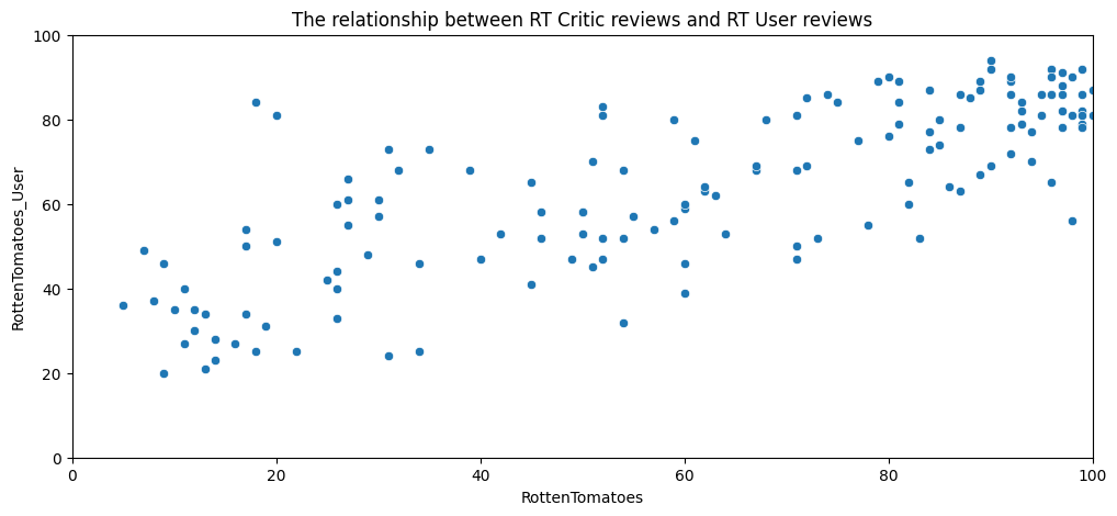
Rotten Tomatoes
Let’s first take a look at Rotten Tomatoes. RT has two sets of reviews, their critics reviews (ratings published by official critics) and user reviews.
#  a scatterplot exploring the relationship between RT Critic reviews and RT User reviews
plt.figure(figsize=(12,5))
sns.scatterplot(data=all_sites, x="RottenTomatoes", y="RottenTomatoes_User")
plt.xlim(0,100)
plt.ylim(0,100)
plt.title("The relationship between RT Critic reviews and RT User reviews")
Text(0.5, 1.0, 'The relationship between RT Critic reviews and RT User reviews')
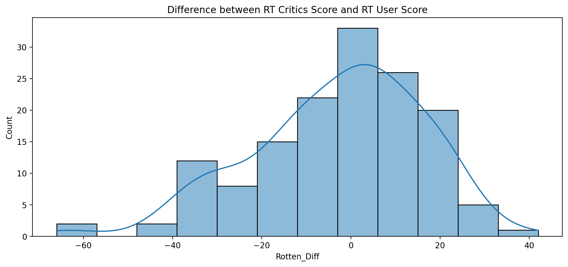
Difference between critics rating and users rating for Rotten Tomatoes - Rotten_Diff
# Difference between critics rating and users rating for Rotten Tomatoes
all_sites["Rotten_Diff"] = all_sites["RottenTomatoes"] - all_sites["RottenTomatoes_User"]
all_sites.head()
| FILM | RottenTomatoes | RottenTomatoes_User | Metacritic | Metacritic_User | IMDB | Metacritic_user_vote_count | IMDB_user_vote_count | Rotten_Diff | |
|---|---|---|---|---|---|---|---|---|---|
| 0 | Avengers: Age of Ultron (2015) | 74 | 86 | 66 | 7.1 | 7.8 | 1330 | 271107 | -12 |
| 1 | Cinderella (2015) | 85 | 80 | 67 | 7.5 | 7.1 | 249 | 65709 | 5 |
| 2 | Ant-Man (2015) | 80 | 90 | 64 | 8.1 | 7.8 | 627 | 103660 | -10 |
| 3 | Do You Believe? (2015) | 18 | 84 | 22 | 4.7 | 5.4 | 31 | 3136 | -66 |
| 4 | Hot Tub Time Machine 2 (2015) | 14 | 28 | 29 | 3.4 | 5.1 | 88 | 19560 | -14 |
Absolute mean difference between the critics rating versus the user rating
# absolute mean difference between the critics rating versus the user rating
all_sites["Rotten_Diff"].abs().mean()
15.095890410958905
# The distribution of the differences between RT Critics Score and RT User Score
plt.figure(figsize=(12,5),dpi=200)
sns.histplot(x=all_sites["Rotten_Diff"], kde=True)
plt.title("Difference between RT Critics Score and RT User Score")
Text(0.5, 1.0, 'Difference between RT Critics Score and RT User Score')
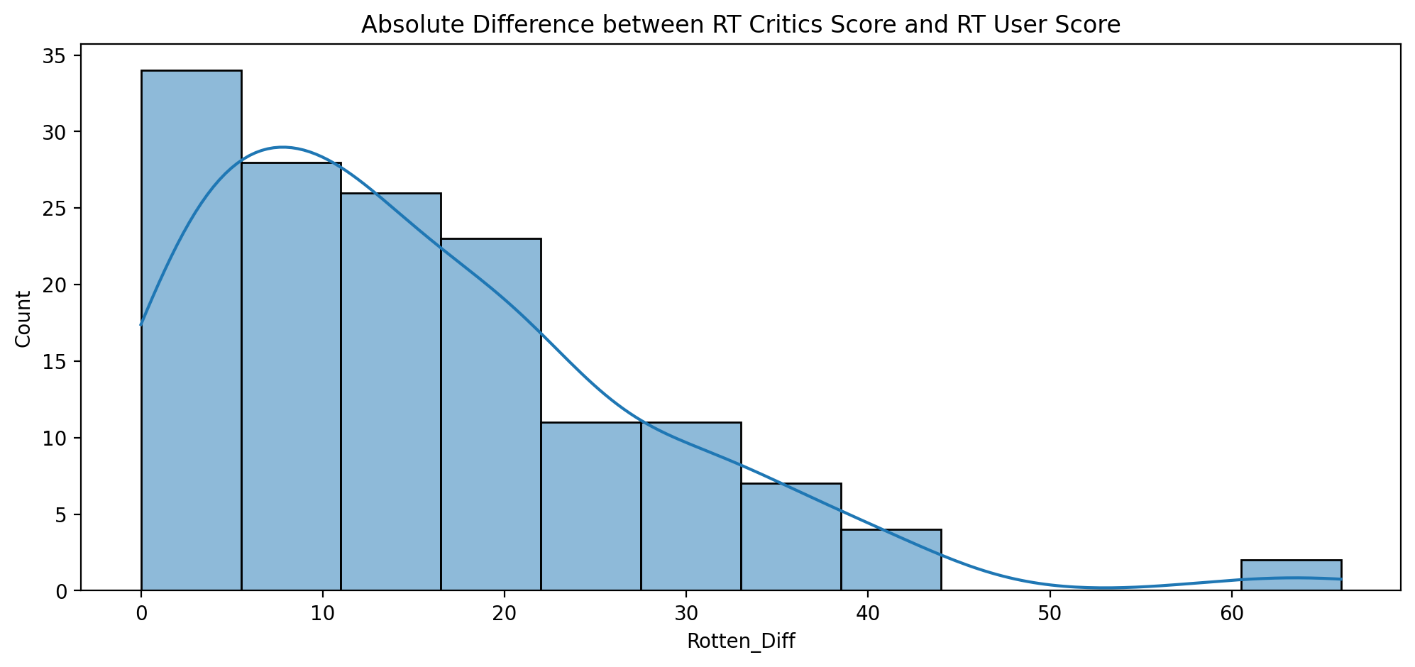
# a distribution showing the absolute value difference between Critics and Users on Rotten Tomatoes
plt.figure(figsize=(12,5),dpi=200)
sns.histplot(x=all_sites["Rotten_Diff"].abs(), kde=True)
plt.title("Absolute Difference between RT Critics Score and RT User Score")
Text(0.5, 1.0, 'Absolute Difference between RT Critics Score and RT User Score')
Top 5 movies users rated higher than critics on average (Users Love but Critics Hate)
# Top 5 movies users rated higher than critics on average
# Users Love but Critics Hate
all_sites.sort_values(by=["Rotten_Diff"])[:5][["FILM", "Rotten_Diff"]]
| FILM | Rotten_Diff | |
|---|---|---|
| 3 | Do You Believe? (2015) | -66 |
| 85 | Little Boy (2015) | -61 |
| 134 | The Longest Ride (2015) | -42 |
| 105 | Hitman: Agent 47 (2015) | -42 |
| 125 | The Wedding Ringer (2015) | -39 |
The top 5 movies critics scores higher than users on average (Critics love, but Users Hate)
# The top 5 movies critics scores higher than users on average
# Critics love, but Users Hate
all_sites.sort_values(by=["Rotten_Diff"], ascending=False)[:5][["FILM", "Rotten_Diff"]]
| FILM | Rotten_Diff | |
|---|---|---|
| 69 | Mr. Turner (2014) | 42 |
| 112 | It Follows (2015) | 31 |
| 115 | While We're Young (2015) | 31 |
| 145 | Kumiko, The Treasure Hunter (2015) | 24 |
| 37 | Welcome to Me (2015) | 24 |
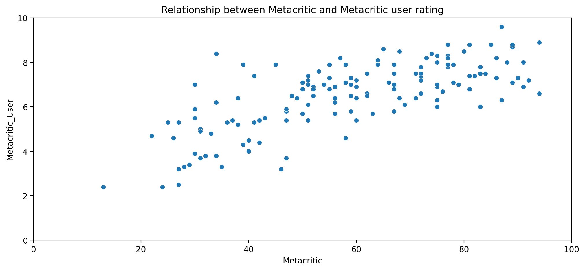
MetaCritic
Now let’s take a quick look at the ratings from MetaCritic. Metacritic also shows an average user rating versus their official displayed rating.
# Metacritic Rating versus the Metacritic User rating
plt.figure(figsize=(12,5),dpi=200)
sns.scatterplot(data=all_sites, x="Metacritic",y="Metacritic_User")
plt.xlim(0,100)
plt.ylim(0,10)
plt.title("Relationship between Metacritic and Metacritic user rating")
Text(0.5, 1.0, 'Relationship between Metacritic and Metacritic user rating')
IMDB
Finally let’s explore IMDB. Notice that both Metacritic and IMDB report back vote counts. Let’s analyze the most popular movies.
# The relationship between vote counts on MetaCritic versus vote counts on IMDB
plt.figure(figsize=(12,5),dpi=200)
sns.scatterplot(data=all_sites, x="Metacritic_user_vote_count",y="IMDB_user_vote_count")
plt.title("The relationship between vote counts on MetaCritic and vote counts on IMDB")
Text(0.5, 1.0, 'The relationship between vote counts on MetaCritic and vote counts on IMDB')
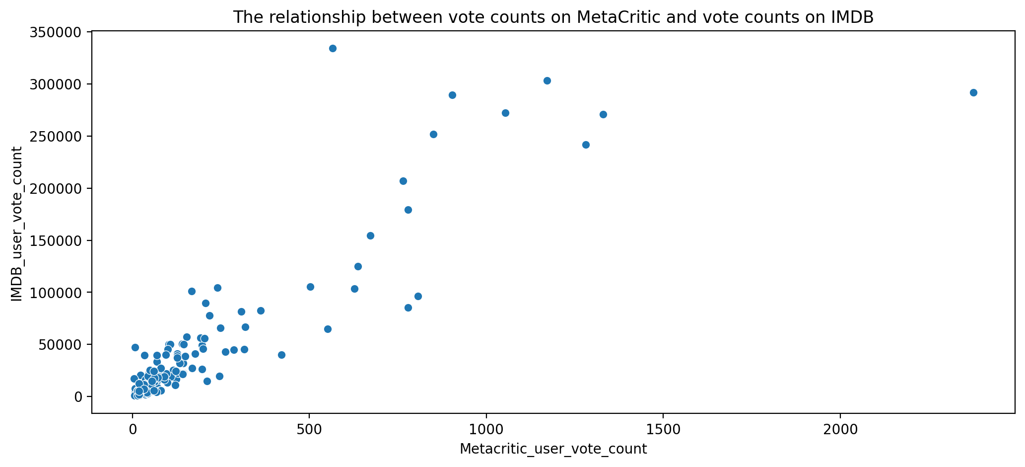
Movie that has the highest IMDB user vote count
# Movie that has the highest IMDB user vote count
all_sites[all_sites["IMDB_user_vote_count"] == all_sites["IMDB_user_vote_count"].max()]
| FILM | RottenTomatoes | RottenTomatoes_User | Metacritic | Metacritic_User | IMDB | Metacritic_user_vote_count | IMDB_user_vote_count | Rotten_Diff | |
|---|---|---|---|---|---|---|---|---|---|
| 14 | The Imitation Game (2014) | 90 | 92 | 73 | 8.2 | 8.1 | 566 | 334164 | -2 |
Movie has the highest Metacritic User Vote count
# Movie has the highest Metacritic User Vote count
all_sites[all_sites["Metacritic_user_vote_count"] == all_sites["Metacritic_user_vote_count"].max()]
| FILM | RottenTomatoes | RottenTomatoes_User | Metacritic | Metacritic_User | IMDB | Metacritic_user_vote_count | IMDB_user_vote_count | Rotten_Diff | |
|---|---|---|---|---|---|---|---|---|---|
| 88 | Mad Max: Fury Road (2015) | 97 | 88 | 89 | 8.7 | 8.3 | 2375 | 292023 | 9 |
Fandago Scores vs. All Sites
Finally let’s begin to explore whether or not Fandango artificially displays higher ratings than warranted to boost ticket sales.
# Inner join to merge together both DataFrames based on the FILM column
df = pd.merge(fandango, all_sites, on="FILM", how="inner")
Merged table structure (all_sites and fandango)
df.head()
| FILM | STARS | RATING | VOTES | Year | STARS_DIFF | RottenTomatoes | RottenTomatoes_User | Metacritic | Metacritic_User | IMDB | Metacritic_user_vote_count | IMDB_user_vote_count | Rotten_Diff | |
|---|---|---|---|---|---|---|---|---|---|---|---|---|---|---|
| 0 | Fifty Shades of Grey (2015) | 4.0 | 3.9 | 34846 | 2015 | 0.1 | 25 | 42 | 46 | 3.2 | 4.2 | 778 | 179506 | -17 |
| 1 | Jurassic World (2015) | 4.5 | 4.5 | 34390 | 2015 | 0.0 | 71 | 81 | 59 | 7.0 | 7.3 | 1281 | 241807 | -10 |
| 2 | American Sniper (2015) | 5.0 | 4.8 | 34085 | 2015 | 0.2 | 72 | 85 | 72 | 6.6 | 7.4 | 850 | 251856 | -13 |
| 3 | Furious 7 (2015) | 5.0 | 4.8 | 33538 | 2015 | 0.2 | 81 | 84 | 67 | 6.8 | 7.4 | 764 | 207211 | -3 |
| 4 | Inside Out (2015) | 4.5 | 4.5 | 15749 | 2015 | 0.0 | 98 | 90 | 94 | 8.9 | 8.6 | 807 | 96252 | 8 |
Table info
df.info()
<class 'pandas.core.frame.DataFrame'>
Int64Index: 145 entries, 0 to 144
Data columns (total 14 columns):
 #   Column                      Non-Null Count  Dtype
---  ------                      --------------  -----
 0   FILM                        145 non-null    object
 1   STARS                       145 non-null    float64
 2   RATING                      145 non-null    float64
 3   VOTES                       145 non-null    int64
 4   Year                        145 non-null    object
 5   STARS_DIFF                  145 non-null    float64
 6   RottenTomatoes              145 non-null    int64
 7   RottenTomatoes_User         145 non-null    int64
 8   Metacritic                  145 non-null    int64
 9   Metacritic_User             145 non-null    float64
 10  IMDB                        145 non-null    float64
 11  Metacritic_user_vote_count  145 non-null    int64
 12  IMDB_user_vote_count        145 non-null    int64
 13  Rotten_Diff                 145 non-null    int64
dtypes: float64(5), int64(7), object(2)
memory usage: 17.0+ KB
Normalizing columns to Fandango STARS and RATINGS 0-5
Notice that RT, Metacritic, and IMDB don’t use a score between 0-5 stars like Fandango does. In order to do a fair comparison, we need to normalize these values so they all fall between 0-5 stars and the relationship between reviews stays the same.
# Normalizing by the current scale level
df["RT_norm"] = df["RottenTomatoes"] / 20
df["RTUser_norm"] = df["RottenTomatoes_User"] / 20
df["Meta_norm"] = df["Metacritic"] / 20
df["MetaUser_norm"] = df["Metacritic_User"] / 2
df["Imdb_norm"] = df["IMDB"] / 2
Merged table with normalized ratings
df = df[["FILM", "STARS","RATING","RT_norm","RTUser_norm","Meta_norm","MetaUser_norm","Imdb_norm"]]
df.head()
| FILM | STARS | RATING | RT_norm | RTUser_norm | Meta_norm | MetaUser_norm | Imdb_norm | |
|---|---|---|---|---|---|---|---|---|
| 0 | Fifty Shades of Grey (2015) | 4.0 | 3.9 | 1.25 | 2.10 | 2.30 | 1.60 | 2.10 |
| 1 | Jurassic World (2015) | 4.5 | 4.5 | 3.55 | 4.05 | 2.95 | 3.50 | 3.65 |
| 2 | American Sniper (2015) | 5.0 | 4.8 | 3.60 | 4.25 | 3.60 | 3.30 | 3.70 |
| 3 | Furious 7 (2015) | 5.0 | 4.8 | 4.05 | 4.20 | 3.35 | 3.40 | 3.70 |
| 4 | Inside Out (2015) | 4.5 | 4.5 | 4.90 | 4.50 | 4.70 | 4.45 | 4.30 |
Comparing Distribution of Scores Across Sites
Now the moment of truth! Does Fandango display abnormally high ratings? We already know it pushs displayed RATING higher than STARS, but are the ratings themselves higher than average?
def move_legend(ax, new_loc, **kws):
    old_legend = ax.legend_
    handles = old_legend.legend_handles
    labels = [t.get_text() for t in old_legend.get_texts()]
    title = old_legend.get_title().get_text()
    ax.legend(handles, labels, loc=new_loc, title=title, **kws)
fig, ax = plt.subplots(figsize=(15,6),dpi=150)
sns.kdeplot(data=df,clip=[0,5],fill=True,palette='Set1',ax=ax)
move_legend(ax, "upper left")
plt.title("Various rating distributions")
Text(0.5, 1.0, 'Various rating distributions')
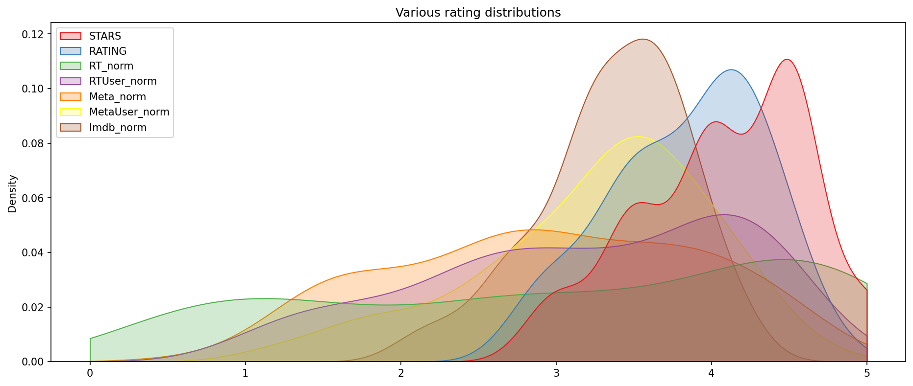
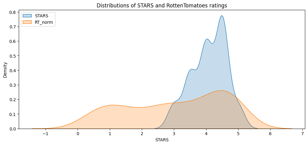
Clearly Fandango has an uneven distribution. We can also see that RT critics have the most uniform distribution. Let’s directly compare these two.
#CODE HERE
plt.figure(figsize=(12,5))
sns.kdeplot(data=df, x="STARS", label="STARS", fill=True)
sns.kdeplot(data=df, x="RT_norm", label="RT_norm", fill=True)
plt.legend(loc='upper left')
plt.title("Distributions of STARS and RottenTomatoes ratings")
Text(0.5, 1.0, 'Distributions of STARS and RottenTomatoes ratings')
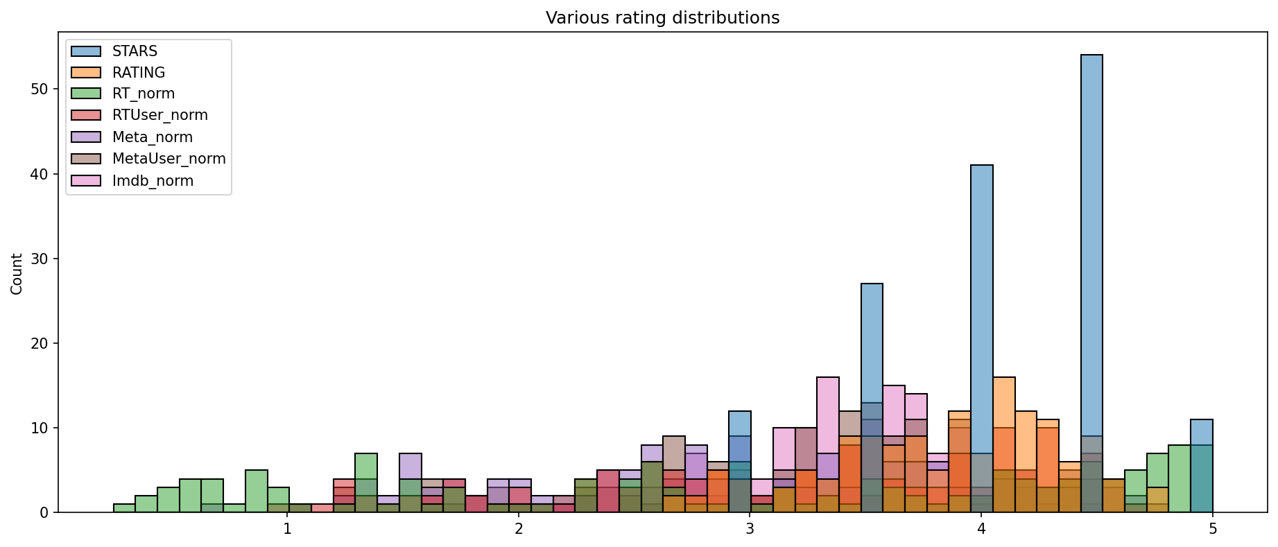
# Histogram plot comparig all normalized scores
plt.subplots(figsize=(15,6),dpi=150)
sns.histplot(df,bins=50)
plt.title("Various rating distributions")
Text(0.5, 1.0, 'Various rating distributions')
# Clustermap visialzation of all normalized scores
sns.clustermap(df[["STARS","RATING","RT_norm","RTUser_norm","Meta_norm","MetaUser_norm","Imdb_norm"]],cmap='magma',col_cluster=False)
plt.title("Clustermap visialzation of all normalized scores")
Text(0.5, 1.0, 'Clustermap visialzation of all normalized scores')
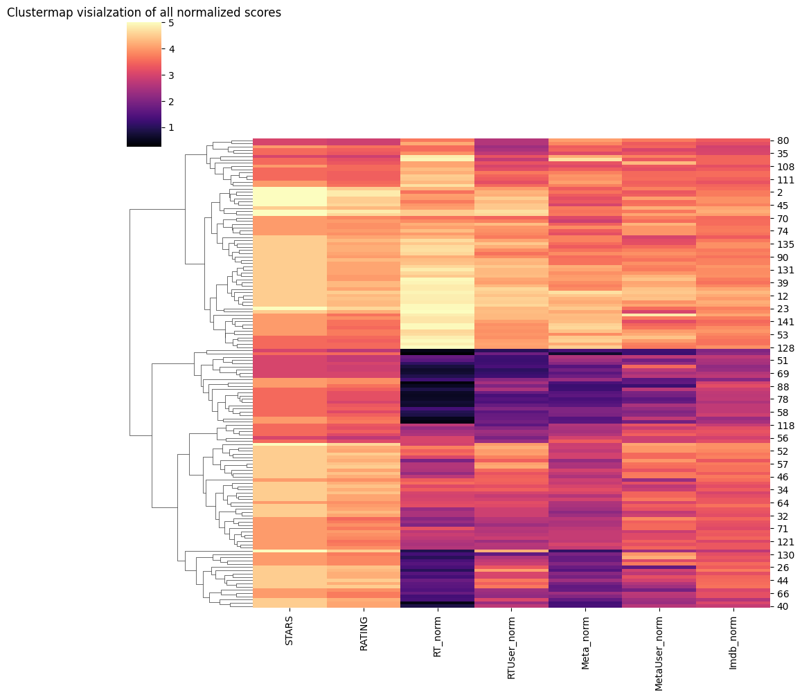
Clearly Fandango is rating movies much higher than other sites, especially considering that it is then displaying a rounded up version of the rating. Let’s examine the top 10 worst movies based off the Rotten Tomatoes Critic Ratings.
The top 10 worst movies based of the Rotten Tomatoes Critics Ratings
df.nsmallest(10,'RT_norm')
| FILM | STARS | RATING | RT_norm | RTUser_norm | Meta_norm | MetaUser_norm | Imdb_norm | |
|---|---|---|---|---|---|---|---|---|
| 49 | Paul Blart: Mall Cop 2 (2015) | 3.5 | 3.5 | 0.25 | 1.80 | 0.65 | 1.20 | 2.15 |
| 84 | Hitman: Agent 47 (2015) | 4.0 | 3.9 | 0.35 | 2.45 | 1.40 | 1.65 | 2.95 |
| 54 | Hot Pursuit (2015) | 4.0 | 3.7 | 0.40 | 1.85 | 1.55 | 1.85 | 2.45 |
| 25 | Taken 3 (2015) | 4.5 | 4.1 | 0.45 | 2.30 | 1.30 | 2.30 | 3.05 |
| 28 | Fantastic Four (2015) | 3.0 | 2.7 | 0.45 | 1.00 | 1.35 | 1.25 | 2.00 |
| 50 | The Boy Next Door (2015) | 4.0 | 3.6 | 0.50 | 1.75 | 1.50 | 2.75 | 2.30 |
| 87 | Unfinished Business (2015) | 3.5 | 3.2 | 0.55 | 1.35 | 1.60 | 1.90 | 2.70 |
| 88 | The Loft (2015) | 4.0 | 3.6 | 0.55 | 2.00 | 1.20 | 1.20 | 3.15 |
| 77 | Seventh Son (2015) | 3.5 | 3.2 | 0.60 | 1.75 | 1.50 | 1.95 | 2.75 |
| 78 | Mortdecai (2015) | 3.5 | 3.2 | 0.60 | 1.50 | 1.35 | 1.60 | 2.75 |
Visualization the distribution of ratings across all sites for the top 10 worst movies.
plt.figure(figsize=(15,6),dpi=150)
worst_films = df.nsmallest(10,'RT_norm').drop('FILM',axis=1)
sns.kdeplot(data=worst_films,clip=[0,5],fill=True,palette='Set1')
plt.title("Ratings for RT Critic's 10 Worst Reviewed Films");
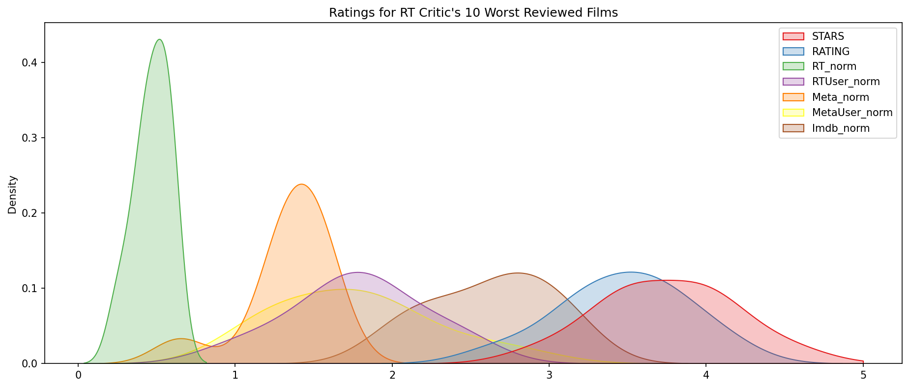

Final thoughts: Wow! Fandango is showing around 3-4 star ratings for films that are clearly bad! Notice the biggest offender, Taken 3!. Fandango is displaying 4.5 stars on their site for a film with an average rating of 1.86 across the other platforms!
Taken 3 rating across platforms
# Taken 3 rating across platforms
df.iloc[25]
FILM             Taken 3 (2015)
STARS                       4.5
RATING                      4.1
RT_norm                    0.45
RTUser_norm                 2.3
Meta_norm                   1.3
MetaUser_norm               2.3
Imdb_norm                  3.05
Name: 25, dtype: object
# Comparison between fandango scores and average scores from all sites
taken3_stars = df.iloc[25]["STARS"]
take3_all_sites_avg = df.iloc[25][["RT_norm", "RTUser_norm", "Meta_norm", "MetaUser_norm", "Imdb_norm"]].mean().round(1)
taken3_all_sites = df.iloc[25][["RT_norm", "RTUser_norm", "Meta_norm", "MetaUser_norm", "Imdb_norm"]]
f"Fandango score for movie 'Taken 3': {taken3_stars}, all sites average score: {take3_all_sites_avg}"
"Fandango score for movie 'Taken 3': 4.5, all sites average score: 1.9"
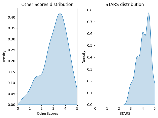
dfhelper = pd.concat([df['RT_norm'], df['RTUser_norm'], df['Meta_norm'], df['MetaUser_norm'], df['Imdb_norm']], axis=1)
dfhelper = dfhelper.stack().reset_index()
dfhelper = dfhelper.rename(columns={0: 'OtherScores'})
x=dfhelper["OtherScores"]
y=df["STARS"]

df_for_ttest = pd.concat([x,y], axis=1)
fig, axes = plt.subplots(nrows=1, ncols=2)

sns.kdeplot(x=x, ax=axes[0], fill=True)
sns.kdeplot(x=y, ax=axes[1], fill=True)

axes[0].set_title("Other Scores distribution", loc="center")
axes[1].set_title("STARS distribution", loc="center")

axes[0].set_xlim(0,5)
axes[1].set_xlim(0,5)
plt.tight_layout()
plt.show()
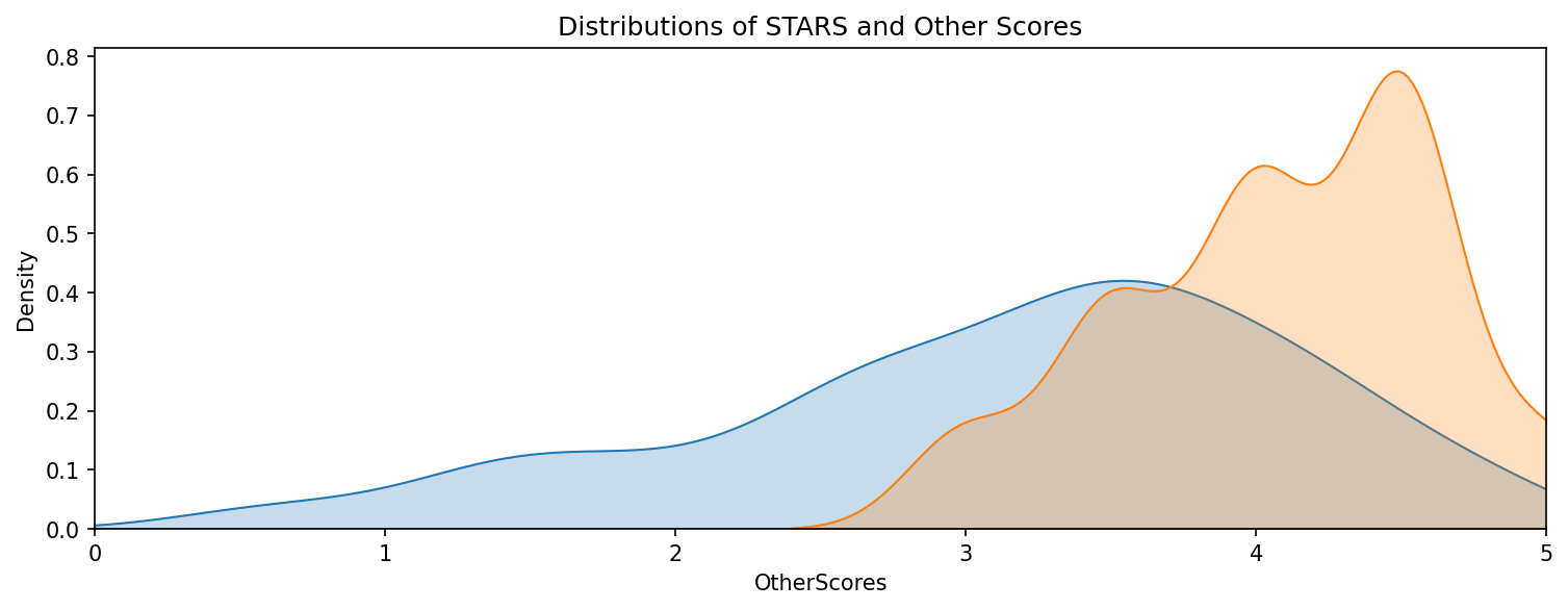
plt.figure(figsize=(12,4),dpi=150)

x=dfhelper["OtherScores"]
y=df["STARS"]

sns.kdeplot(x=x, fill=True)
sns.kdeplot(x=y, fill=True)

plt.xlim(0,5)
plt.title("Distributions of STARS and Other Scores", loc="center")
Text(0.5, 1.0, 'Distributions of STARS and Other Scores')
# Import the library
import scipy.stats as stats

# Perform the two sample t-test with equal variances
t, p = stats.ttest_ind(a=dfhelper["OtherScores"], b=df["STARS"], equal_var=False)
m_Stars = x.mean()
m_OtherScores = y.mean()

f"Average Stars = {m_Stars.round(2)}, Average OtherScores = {m_OtherScores.round(2)}, t-value = {t.round(2)}, p < {p.round(2)}"
'Average Stars = 3.15, Average OtherScores = 4.09, t-value = -15.91, p < 0.0'
"almost 1 whole point away of each other"
'almost 1 whole point away of each other'
What have we learned?
The difference of 1 point in the rating score can play a big role in the perception of the quality against the common rating standard (on a scale 1-5). One point of difference in the rating score obviously made people suspicious of investigating the data quality.
This analysis made clear how questioning can discover interesting trends in data.
Bottom line - Do not be too obvious when biasing information in your direction!
Remaining questions
- What is the differential threshold when people will notice the trend between the distributions?
- In other words, when people will notice that Fendango rates the moves more favourably towards (certain) movies than the other platforms?
- What is the optimal rate to manipulate movie (or other) ratings over time so the manipulations stay disguised, but effective?